Introduction to NeuralHydrology
Before we start
This tutorial is rendered from a Jupyter notebook that is hosted on GitHub. If you want to run the code yourself, you can find the notebook and configuration files here.
To be able to run this notebook locally, you need to download the publicly available CAMELS US rainfall-runoff dataset. See the Data Prerequisites Tutorial for a detailed description on where to download the data and how to structure your local dataset folder. You will also need to follow the installation instructions (the easiest option if you don’t plan to implement your own models/datasets is
pip install neuralhydrology; for other options refer to the installation instructions).
The Python package NeuralHydrology was was developed with a strong focus on research. The main application area is hydrology, however, in principle the code can be used with any data. To allow fast iteration of research ideas, we tried to develop the package as modular as possible so that new models, new data sets, new loss functions, new regularizations, new metrics etc. can be integrated with minor effort.
There are two different ways to use this package:
From the terminal, making use of some high-level entry points (such as
nh-runandnh-schedule-runs)From any other Python file or Jupyter Notebook, using NeuralHydrology’s API
In this tutorial, we will give a very short overview of the two different modes.
Both approaches require a configuration file. These are .yml files which define the entire run configuration (such as data set, basins, data periods, model specifications, etc.). A full list of config arguments is listed in the documentation and we highly recommend to check this page and read the documentation carefully. There is a lot that you can do with this Python package and we can’t cover everything in
tutorials.
For every run that you start, a new folder will be created. This folder is used to store the model and optimizer checkpoints, train data means/stds (needed for scaling during inference), tensorboard log file (can be used to monitor and compare training runs visually), validation results (optionally) and training progress figures (optionally, e.g., model predictions and observations for n random basins). During inference, the evaluation results will also be stored in this directory (e.g., test period results).
TensorBoard logging
By default, the training progress is logged in TensorBoard files (add log_tensorboard: False to the config to disable TensorBoard logging). If you installed a Python environment from one of our environment files, you have TensorBoard already installed. If not, you can install TensorBoard with:
pip install tensorboard
To start the TensorBoard dashboard, run:
tensorboard --logdir /path/to/run-dir
You can also visualize multiple runs at once if you point the --logdir to the parent directory (useful for model intercomparison)
File logging
In addition to TensorBoard, you will always find a file called output.log in the run directory. This file is a dump of the console output you see during training and evaluation.
Using NeuralHydrology from the Terminal
nh-run
Given a run configuration file, you can use the bash command nh-run to train/evaluate a model. To train a model, use
nh-run train --config-file path/to/config.yml
to evaluate the model after training, use
nh-run evaluate --run-dir path/to/run-directory
nh-schedule-runs
If you want to train/evaluate multiple models on different GPUs, you can use the nh-schedule-runs command. This tool automatically distributes runs across GPUs and starts a new one, whenever one run finishes.
Calling nh-schedule-runs in train mode will train one model for each .yml file in a directory (or its sub-directories).
nh-schedule-runs train --directory /path/to/config-dir --runs-per-gpu 2 --gpu_ids 0 1 2 3
Use -runs-per-gpu to define the number of models that are simultaneously trained on a single GPU (2 in this case) and --gpu-ids to define which GPUs will be used (numbers are ids according to nvidia-smi). In this example, 8 models will train simultaneously on 4 different GPUs.
Calling nh-schedule-runs in evaluate mode will evaluate all models in all run directories in a given root directory.
nh-schedule-runs evaluate --directory /path/to/parent-run-dir/ --runs-per-gpu 2 --gpu_ids 0 1 2 3
API usage
Besides the command line tools, you can also use the NeuralHydrology package just like any other Python package by importing its modules, classes, or functions.
This can be helpful for exploratory studies with trained models, but also if you want to use some of the functions or classes within a different codebase.
Look at the API Documentation for a full list of functions/classes you could use.
The following example shows how to train and evaluate a model via the API.
[1]:
import pickle
from pathlib import Path

import matplotlib.pyplot as plt
import torch
from neuralhydrology.evaluation import metrics
from neuralhydrology.nh_run import start_run, eval_run
Train a model for a single config file
Note
The config file assumes that the CAMELS US dataset is stored under
data/CAMELS_US(relative to the main directory of this repository) or a symbolic link exists at this location. Make sure that this folder contains the required subdirectoriesbasin_mean_forcing,usgs_streamflowandcamels_attributes_v2.0. If your data is stored at a different location and you can’t or don’t want to create a symbolic link, you will need to change thedata_dirargument in the1_basin.ymlconfig file that is located in the same directory as this notebook.By default, the config (
1_basin.yml) assumes that you have a CUDA-capable NVIDIA GPU (see config argumentdevice). In case you don’t have any or you have one but want to train on the CPU, you can either change the config argument todevice: cpuor passgpu=-1to thestart_run()function.If you want to train on MacOS devices with Metal programming framework which enables high-performance training on GPU for MacOS, change the config argument to
device: mpsand don’t pass thegpuargument to thestart_run()function.
[2]:
# by default we assume that you have at least one CUDA-capable NVIDIA GPU or MacOS with Metal support
if torch.cuda.is_available() or torch.backends.mps.is_available():
    start_run(config_file=Path("1_basin.yml"))

# fall back to CPU-only mode
else:
    start_run(config_file=Path("1_basin.yml"), gpu=-1)
2022-01-05 21:49:45,640: Logging to /home/frederik/Projects/neuralhydrology/examples/01-Introduction/runs/test_run_0501_214945/output.log initialized.
2022-01-05 21:49:45,641: ### Folder structure created at /home/frederik/Projects/neuralhydrology/examples/01-Introduction/runs/test_run_0501_214945
2022-01-05 21:49:45,641: ### Run configurations for test_run
2022-01-05 21:49:45,641: experiment_name: test_run
2022-01-05 21:49:45,641: train_basin_file: 1_basin.txt
2022-01-05 21:49:45,642: validation_basin_file: 1_basin.txt
2022-01-05 21:49:45,642: test_basin_file: 1_basin.txt
2022-01-05 21:49:45,642: train_start_date: 1999-10-01 00:00:00
2022-01-05 21:49:45,643: train_end_date: 2008-09-30 00:00:00
2022-01-05 21:49:45,643: validation_start_date: 1980-10-01 00:00:00
2022-01-05 21:49:45,643: validation_end_date: 1989-09-30 00:00:00
2022-01-05 21:49:45,644: test_start_date: 1989-10-01 00:00:00
2022-01-05 21:49:45,644: test_end_date: 1999-09-30 00:00:00
2022-01-05 21:49:45,644: device: cuda:0
2022-01-05 21:49:45,644: validate_every: 3
2022-01-05 21:49:45,645: validate_n_random_basins: 1
2022-01-05 21:49:45,645: metrics: ['NSE']
2022-01-05 21:49:45,645: model: cudalstm
2022-01-05 21:49:45,645: head: regression
2022-01-05 21:49:45,645: output_activation: linear
2022-01-05 21:49:45,646: hidden_size: 20
2022-01-05 21:49:45,646: initial_forget_bias: 3
2022-01-05 21:49:45,646: output_dropout: 0.4
2022-01-05 21:49:45,647: optimizer: Adam
2022-01-05 21:49:45,647: loss: MSE
2022-01-05 21:49:45,647: learning_rate: {0: 0.01, 30: 0.005, 40: 0.001}
2022-01-05 21:49:45,647: batch_size: 256
2022-01-05 21:49:45,647: epochs: 50
2022-01-05 21:49:45,648: clip_gradient_norm: 1
2022-01-05 21:49:45,648: predict_last_n: 1
2022-01-05 21:49:45,648: seq_length: 365
2022-01-05 21:49:45,648: num_workers: 8
2022-01-05 21:49:45,649: log_interval: 5
2022-01-05 21:49:45,649: log_tensorboard: True
2022-01-05 21:49:45,649: log_n_figures: 1
2022-01-05 21:49:45,649: save_weights_every: 1
2022-01-05 21:49:45,649: dataset: camels_us
2022-01-05 21:49:45,650: data_dir: ../../data/CAMELS_US
2022-01-05 21:49:45,650: forcings: ['maurer', 'daymet', 'nldas']
2022-01-05 21:49:45,650: dynamic_inputs: ['PRCP(mm/day)_nldas', 'PRCP(mm/day)_maurer', 'prcp(mm/day)_daymet', 'srad(W/m2)_daymet', 'tmax(C)_daymet', 'tmin(C)_daymet', 'vp(Pa)_daymet']
2022-01-05 21:49:45,650: target_variables: ['QObs(mm/d)']
2022-01-05 21:49:45,651: clip_targets_to_zero: ['QObs(mm/d)']
2022-01-05 21:49:45,651: number_of_basins: 1
2022-01-05 21:49:45,651: run_dir: /home/frederik/Projects/neuralhydrology/examples/01-Introduction/runs/test_run_0501_214945
2022-01-05 21:49:45,651: train_dir: /home/frederik/Projects/neuralhydrology/examples/01-Introduction/runs/test_run_0501_214945/train_data
2022-01-05 21:49:45,651: img_log_dir: /home/frederik/Projects/neuralhydrology/examples/01-Introduction/runs/test_run_0501_214945/img_log
2022-01-05 21:49:45,709: ### Device cuda:0 will be used for training
2022-01-05 21:49:47,226: Loading basin data into xarray data set.
100%|██████████| 1/1 [00:00<00:00, 15.40it/s]
2022-01-05 21:49:47,296: Create lookup table and convert to pytorch tensor
100%|██████████| 1/1 [00:00<00:00,  1.14it/s]
# Epoch 1: 100%|██████████| 13/13 [00:00<00:00, 34.14it/s, Loss: 0.1480]
2022-01-05 21:49:48,653: Epoch 1 average loss: 0.36545397914372957
# Epoch 2: 100%|██████████| 13/13 [00:00<00:00, 35.94it/s, Loss: 0.2337]
2022-01-05 21:49:49,018: Epoch 2 average loss: 0.24019309878349304
# Epoch 3: 100%|██████████| 13/13 [00:00<00:00, 36.27it/s, Loss: 0.1639]
2022-01-05 21:49:49,380: Epoch 3 average loss: 0.1756665316911844
# Validation: 100%|██████████| 1/1 [00:00<00:00,  2.92it/s]
2022-01-05 21:49:49,872: Epoch 3 average validation loss: 0.15335 -- Median validation metrics: NSE: 0.64457
# Epoch 4: 100%|██████████| 13/13 [00:00<00:00, 38.55it/s, Loss: 0.1220]
2022-01-05 21:49:50,211: Epoch 4 average loss: 0.13774388627364084
# Epoch 5: 100%|██████████| 13/13 [00:00<00:00, 36.56it/s, Loss: 0.1014]
2022-01-05 21:49:50,571: Epoch 5 average loss: 0.12395260884211613
# Epoch 6: 100%|██████████| 13/13 [00:00<00:00, 38.48it/s, Loss: 0.0758]
2022-01-05 21:49:50,912: Epoch 6 average loss: 0.10742208590874305
# Validation: 100%|██████████| 1/1 [00:00<00:00, 10.64it/s]
2022-01-05 21:49:51,151: Epoch 6 average validation loss: 0.12586 -- Median validation metrics: NSE: 0.71063
# Epoch 7: 100%|██████████| 13/13 [00:00<00:00, 38.06it/s, Loss: 0.0970]
2022-01-05 21:49:51,496: Epoch 7 average loss: 0.09842771377701026
# Epoch 8: 100%|██████████| 13/13 [00:00<00:00, 38.88it/s, Loss: 0.0730]
2022-01-05 21:49:51,834: Epoch 8 average loss: 0.08783119544386864
# Epoch 9: 100%|██████████| 13/13 [00:00<00:00, 36.36it/s, Loss: 0.0964]
2022-01-05 21:49:52,195: Epoch 9 average loss: 0.08482636855198787
# Validation: 100%|██████████| 1/1 [00:00<00:00, 11.19it/s]
2022-01-05 21:49:52,426: Epoch 9 average validation loss: 0.11695 -- Median validation metrics: NSE: 0.73042
# Epoch 10: 100%|██████████| 13/13 [00:00<00:00, 21.60it/s, Loss: 0.1034]
2022-01-05 21:49:53,031: Epoch 10 average loss: 0.08333522654496707
# Epoch 11: 100%|██████████| 13/13 [00:00<00:00, 21.26it/s, Loss: 0.0462]
2022-01-05 21:49:53,646: Epoch 11 average loss: 0.08473585316768059
# Epoch 12: 100%|██████████| 13/13 [00:00<00:00, 21.14it/s, Loss: 0.0602]
2022-01-05 21:49:54,266: Epoch 12 average loss: 0.08158419768397625
# Validation: 100%|██████████| 1/1 [00:00<00:00,  4.69it/s]
2022-01-05 21:49:54,620: Epoch 12 average validation loss: 0.10083 -- Median validation metrics: NSE: 0.76347
# Epoch 13: 100%|██████████| 13/13 [00:00<00:00, 34.60it/s, Loss: 0.1676]
2022-01-05 21:49:54,998: Epoch 13 average loss: 0.0712348775794873
# Epoch 14: 100%|██████████| 13/13 [00:00<00:00, 34.43it/s, Loss: 0.1158]
2022-01-05 21:49:55,379: Epoch 14 average loss: 0.06913305217256913
# Epoch 15: 100%|██████████| 13/13 [00:00<00:00, 36.80it/s, Loss: 0.1342]
2022-01-05 21:49:55,737: Epoch 15 average loss: 0.08255905486070193
# Validation: 100%|██████████| 1/1 [00:00<00:00,  9.50it/s]
2022-01-05 21:49:55,986: Epoch 15 average validation loss: 0.09562 -- Median validation metrics: NSE: 0.77740
# Epoch 16: 100%|██████████| 13/13 [00:00<00:00, 37.33it/s, Loss: 0.0399]
2022-01-05 21:49:56,336: Epoch 16 average loss: 0.07054153657876529
# Epoch 17: 100%|██████████| 13/13 [00:00<00:00, 36.75it/s, Loss: 0.0531]
2022-01-05 21:49:56,693: Epoch 17 average loss: 0.060455145744177013
# Epoch 18: 100%|██████████| 13/13 [00:00<00:00, 37.59it/s, Loss: 0.0362]
2022-01-05 21:49:57,042: Epoch 18 average loss: 0.05935263576415869
# Validation: 100%|██████████| 1/1 [00:00<00:00, 10.32it/s]
2022-01-05 21:49:57,282: Epoch 18 average validation loss: 0.09405 -- Median validation metrics: NSE: 0.78156
# Epoch 19: 100%|██████████| 13/13 [00:00<00:00, 37.43it/s, Loss: 0.0639]
2022-01-05 21:49:57,632: Epoch 19 average loss: 0.06714180197853309
# Epoch 20: 100%|██████████| 13/13 [00:00<00:00, 37.65it/s, Loss: 0.0825]
2022-01-05 21:49:57,981: Epoch 20 average loss: 0.06650257855653763
# Epoch 21: 100%|██████████| 13/13 [00:00<00:00, 37.03it/s, Loss: 0.0526]
2022-01-05 21:49:58,336: Epoch 21 average loss: 0.06315624656585547
# Validation: 100%|██████████| 1/1 [00:00<00:00, 10.96it/s]
2022-01-05 21:49:58,570: Epoch 21 average validation loss: 0.10051 -- Median validation metrics: NSE: 0.76904
# Epoch 22: 100%|██████████| 13/13 [00:00<00:00, 36.95it/s, Loss: 0.1066]
2022-01-05 21:49:58,924: Epoch 22 average loss: 0.0605762406037404
# Epoch 23: 100%|██████████| 13/13 [00:00<00:00, 33.68it/s, Loss: 0.0392]
2022-01-05 21:49:59,314: Epoch 23 average loss: 0.05911955552605482
# Epoch 24: 100%|██████████| 13/13 [00:00<00:00, 36.31it/s, Loss: 0.0509]
2022-01-05 21:49:59,675: Epoch 24 average loss: 0.0670818855556158
# Validation: 100%|██████████| 1/1 [00:00<00:00, 10.91it/s]
2022-01-05 21:49:59,913: Epoch 24 average validation loss: 0.09044 -- Median validation metrics: NSE: 0.79029
# Epoch 25: 100%|██████████| 13/13 [00:00<00:00, 37.54it/s, Loss: 0.0617]
2022-01-05 21:50:00,261: Epoch 25 average loss: 0.060912144012176074
# Epoch 26: 100%|██████████| 13/13 [00:00<00:00, 36.89it/s, Loss: 0.0716]
2022-01-05 21:50:00,617: Epoch 26 average loss: 0.06060298790152256
# Epoch 27: 100%|██████████| 13/13 [00:00<00:00, 37.31it/s, Loss: 0.0437]
2022-01-05 21:50:00,970: Epoch 27 average loss: 0.0542260123273501
# Validation: 100%|██████████| 1/1 [00:00<00:00, 11.24it/s]
2022-01-05 21:50:01,198: Epoch 27 average validation loss: 0.09302 -- Median validation metrics: NSE: 0.78432
# Epoch 28: 100%|██████████| 13/13 [00:00<00:00, 37.73it/s, Loss: 0.0617]
2022-01-05 21:50:01,545: Epoch 28 average loss: 0.05370813608169556
# Epoch 29: 100%|██████████| 13/13 [00:00<00:00, 37.16it/s, Loss: 0.0597]
2022-01-05 21:50:01,898: Epoch 29 average loss: 0.051912508331812345
2022-01-05 21:50:01,900: Setting learning rate to 0.005
# Epoch 30: 100%|██████████| 13/13 [00:00<00:00, 36.64it/s, Loss: 0.0424]
2022-01-05 21:50:02,256: Epoch 30 average loss: 0.049096258787008434
# Validation: 100%|██████████| 1/1 [00:00<00:00, 10.78it/s]
2022-01-05 21:50:02,492: Epoch 30 average validation loss: 0.08305 -- Median validation metrics: NSE: 0.80648
# Epoch 31: 100%|██████████| 13/13 [00:00<00:00, 36.40it/s, Loss: 0.1244]
2022-01-05 21:50:02,851: Epoch 31 average loss: 0.05618327999344239
# Epoch 32: 100%|██████████| 13/13 [00:00<00:00, 35.67it/s, Loss: 0.0478]
2022-01-05 21:50:03,219: Epoch 32 average loss: 0.05339241744234012
# Epoch 33: 100%|██████████| 13/13 [00:00<00:00, 35.03it/s, Loss: 0.0618]
2022-01-05 21:50:03,594: Epoch 33 average loss: 0.04871770252402012
# Validation: 100%|██████████| 1/1 [00:00<00:00, 11.17it/s]
2022-01-05 21:50:03,826: Epoch 33 average validation loss: 0.08549 -- Median validation metrics: NSE: 0.80153
# Epoch 34: 100%|██████████| 13/13 [00:00<00:00, 33.52it/s, Loss: 0.0388]
2022-01-05 21:50:04,216: Epoch 34 average loss: 0.055069693292562776
# Epoch 35: 100%|██████████| 13/13 [00:00<00:00, 35.24it/s, Loss: 0.0782]
2022-01-05 21:50:04,588: Epoch 35 average loss: 0.054258897327459775
# Epoch 36: 100%|██████████| 13/13 [00:00<00:00, 36.13it/s, Loss: 0.0345]
2022-01-05 21:50:04,952: Epoch 36 average loss: 0.05193230452445837
# Validation: 100%|██████████| 1/1 [00:00<00:00, 10.69it/s]
2022-01-05 21:50:05,190: Epoch 36 average validation loss: 0.08896 -- Median validation metrics: NSE: 0.79330
# Epoch 37: 100%|██████████| 13/13 [00:00<00:00, 35.31it/s, Loss: 0.0359]
2022-01-05 21:50:05,561: Epoch 37 average loss: 0.04444875038014008
# Epoch 38: 100%|██████████| 13/13 [00:00<00:00, 37.80it/s, Loss: 0.0514]
2022-01-05 21:50:05,908: Epoch 38 average loss: 0.05264786802805387
# Epoch 39: 100%|██████████| 13/13 [00:00<00:00, 37.35it/s, Loss: 0.0376]
2022-01-05 21:50:06,260: Epoch 39 average loss: 0.049682121437329516
# Validation: 100%|██████████| 1/1 [00:00<00:00, 11.51it/s]
2022-01-05 21:50:06,490: Epoch 39 average validation loss: 0.08265 -- Median validation metrics: NSE: 0.80724
2022-01-05 21:50:06,491: Setting learning rate to 0.001
# Epoch 40: 100%|██████████| 13/13 [00:00<00:00, 35.86it/s, Loss: 0.0453]
2022-01-05 21:50:06,856: Epoch 40 average loss: 0.050179240508721426
# Epoch 41: 100%|██████████| 13/13 [00:00<00:00, 36.23it/s, Loss: 0.0360]
2022-01-05 21:50:07,219: Epoch 41 average loss: 0.04854901335560358
# Epoch 42: 100%|██████████| 13/13 [00:00<00:00, 35.66it/s, Loss: 0.0315]
2022-01-05 21:50:07,587: Epoch 42 average loss: 0.04618765786290169
# Validation: 100%|██████████| 1/1 [00:00<00:00, 10.21it/s]
2022-01-05 21:50:07,826: Epoch 42 average validation loss: 0.08838 -- Median validation metrics: NSE: 0.79419
# Epoch 43: 100%|██████████| 13/13 [00:00<00:00, 35.91it/s, Loss: 0.0380]
2022-01-05 21:50:08,190: Epoch 43 average loss: 0.047364794864104345
# Epoch 44: 100%|██████████| 13/13 [00:00<00:00, 37.04it/s, Loss: 0.0483]
2022-01-05 21:50:08,545: Epoch 44 average loss: 0.04533060926657457
# Epoch 45: 100%|██████████| 13/13 [00:00<00:00, 35.75it/s, Loss: 0.0440]
2022-01-05 21:50:08,912: Epoch 45 average loss: 0.042340777527827486
# Validation: 100%|██████████| 1/1 [00:00<00:00, 10.76it/s]
2022-01-05 21:50:09,151: Epoch 45 average validation loss: 0.08624 -- Median validation metrics: NSE: 0.79918
# Epoch 46: 100%|██████████| 13/13 [00:00<00:00, 36.26it/s, Loss: 0.0221]
2022-01-05 21:50:09,512: Epoch 46 average loss: 0.04203573757639298
# Epoch 47: 100%|██████████| 13/13 [00:00<00:00, 36.94it/s, Loss: 0.0394]
2022-01-05 21:50:09,867: Epoch 47 average loss: 0.043037718448501364
# Epoch 48: 100%|██████████| 13/13 [00:00<00:00, 36.40it/s, Loss: 0.0452]
2022-01-05 21:50:10,228: Epoch 48 average loss: 0.04290855618623587
# Validation: 100%|██████████| 1/1 [00:00<00:00, 10.98it/s]
2022-01-05 21:50:10,467: Epoch 48 average validation loss: 0.08623 -- Median validation metrics: NSE: 0.79856
# Epoch 49: 100%|██████████| 13/13 [00:00<00:00, 35.64it/s, Loss: 0.0470]
2022-01-05 21:50:10,834: Epoch 49 average loss: 0.04451469160043276
# Epoch 50: 100%|██████████| 13/13 [00:00<00:00, 36.37it/s, Loss: 0.0370]
2022-01-05 21:50:11,196: Epoch 50 average loss: 0.04601523423424134
Evaluate run on test set
The run directory that needs to be specified for evaluation is printed in the output log above. Since the folder name is created dynamically (including the date and time of the start of the run) you will need to change the run_dir argument according to your local directory name. By default, it will use the same device as during the training process.
[3]:
run_dir = Path("runs/test_run_0501_214945")
eval_run(run_dir=run_dir, period="test")
2022-01-05 21:53:26,501: Using the model weights from runs/test_run_0501_214945/model_epoch050.pt
# Evaluation: 100%|██████████| 1/1 [00:00<00:00,  5.20it/s]
2022-01-05 21:53:26,697: Stored results at runs/test_run_0501_214945/test/model_epoch050/test_results.p
Load and inspect model predictions
Next, we load the results file and compare the model predictions with observations. The results file is always a pickled dictionary with one key per basin (even for a single basin). The next-lower dictionary level is the temporal resolution of the predictions. In this case, we trained a model only on daily data (‘1D’). Within the temporal resolution, the next-lower dictionary level are xr(an xarray Dataset that contains observations and predictions), as well as one key for each metric that
was specified in the config file.
[4]:
with open(run_dir / "test" / "model_epoch050" / "test_results.p", "rb") as fp:
    results = pickle.load(fp)

results.keys()
[4]:
dict_keys(['01022500'])
The data variables in the xarray Dataset are named according to the name of the target variables, with suffix _obs for the observations and suffix _sim for the simulations.
[5]:
results['01022500']['1D']['xr']
[5]:
<xarray.Dataset>
Dimensions:         (date: 3652, time_step: 1)
Coordinates:
  * date            (date) datetime64[ns] 1989-10-01 1989-10-02 ... 1999-09-30
  * time_step       (time_step) int64 0
Data variables:
    QObs(mm/d)_obs  (date, time_step) float32 0.6203 0.5537 ... 1.182 0.9992
QObs(mm/d)_sim (date, time_step) float32 0.5518 0.4252 ... 1.842 1.515- date: 3652
- time_step: 1
- date(date)datetime64[ns]1989-10-01 ... 1999-09-30
array(['1989-10-01T00:00:00.000000000', '1989-10-02T00:00:00.000000000', '1989-10-03T00:00:00.000000000', ..., '1999-09-28T00:00:00.000000000', '1999-09-29T00:00:00.000000000', '1999-09-30T00:00:00.000000000'], dtype='datetime64[ns]') - time_step(time_step)int640
array([0])
- QObs(mm/d)_obs(date, time_step)float320.6203 0.5537 ... 1.182 0.9992
array([[0.62030745], [0.5536971 ], [0.7118964 ], ..., [1.4529347 ], [1.1823308 ], [0.9991529 ]], dtype=float32) - QObs(mm/d)_sim(date, time_step)float320.5518 0.4252 ... 1.842 1.515
array([[0.55176044],
       [0.42521405],
       [0.7064749 ],
       ...,
       [2.287218  ],
       [1.8419595 ],
       [1.5153995 ]], dtype=float32)
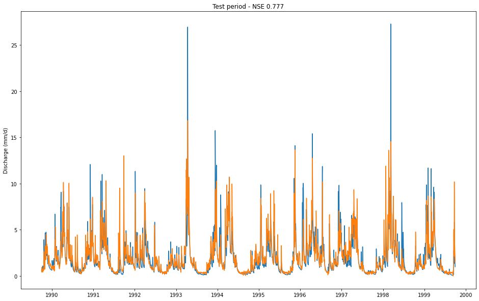
Let’s plot the model predictions vs. the observations
[6]:
# extract observations and simulations
qobs = results['01022500']['1D']['xr']['QObs(mm/d)_obs']
qsim = results['01022500']['1D']['xr']['QObs(mm/d)_sim']

fig, ax = plt.subplots(figsize=(16,10))
ax.plot(qobs['date'], qobs)
ax.plot(qsim['date'], qsim)
ax.set_ylabel("Discharge (mm/d)")
ax.set_title(f"Test period - NSE {results['01022500']['1D']['NSE']:.3f}")
[6]:
Text(0.5, 1.0, 'Test period - NSE 0.777')
Next, we are going to compute all metrics that are implemented in the NeuralHydrology package. You will find additional hydrological signatures implemented in neuralhydrology.evaluation.signatures.
[7]:
values = metrics.calculate_all_metrics(qobs.isel(time_step=-1), qsim.isel(time_step=-1))
for key, val in values.items():
    print(f"{key}: {val:.3f}")
NSE: 0.777
MSE: 1.099
RMSE: 1.048
KGE: 0.850
Alpha-NSE: 0.921
Beta-NSE: 0.048
Pearson-r: 0.883
FHV: -9.371
FMS: -2.198
FLV: -877.436
Peak-Timing: 0.174