CustomLSTM: Inspecting LSTM States and Activations
Before we start
This tutorial is rendered from a Jupyter notebook that is hosted on GitHub. If you want to run the code yourself, you can find the notebook and configuration files here.
To be able to run this notebook locally, you need to download the publicly available CAMELS US rainfall-runoff dataset. See the Data Prerequisites Tutorial for a detailed description on where to download the data and how to structure your local dataset folder.
This tutorial shows how to use CustomLSTM to inspect the states and activations of a trained LSTM. In previous publications, we have seen that the internals of LSTM seem to resemble physically meaningful quantities. For instance, this publication found cells that are highly correlated to snow water equivalent (SWE), even though the LSTM had never seen SWE data during training. While CudaLSTM is great for fast training
of models, it limits the insights we can draw from model internals such as states and activations. This is where CustomLSTM comes into play: CustomLSTM is another LSTM implementation that is much slower but that can return much more information on cell/hidden states and activations.
To train an LSTM model, you’ll always want to use CudaLSTM since it makes use of PyTorch’s pre-implemented LSTM with all its optimizations. Therefore, it’s way faster than anything we could build ourselves. Since CustomLSTM is slower than CudaLSTM, the usual workflow is:
train a
CudaLSTMcopy the
CudaLSTMweights into aCustomLSTManalyze the states/activations in the
CustomLSTM
[1]:
from pathlib import Path
from typing import Dict

import matplotlib.pyplot as plt
import pandas as pd
import torch
from torch.utils.data import DataLoader

from neuralhydrology.datasetzoo import get_dataset, camelsus
from neuralhydrology.datautils.utils import load_scaler
from neuralhydrology.modelzoo.cudalstm import CudaLSTM
from neuralhydrology.modelzoo.customlstm import CustomLSTM
from neuralhydrology.nh_run import start_run
from neuralhydrology.utils.config import Config
To start, let’s train a “normal” LSTM (i.e., a CudaLSTM), just like we did in the introduction tutorial. (Again, for quick results, we train the model on a single basin. If you actually care about good predictions, don’t do this. Train one model on lots of basins combined.).
Note
The config file assumes that the CAMELS US dataset is stored under
data/CAMELS_US(relative to the main directory of this repository) or a symbolic link exists at this location. Make sure that this folder contains the required subdirectoriesbasin_mean_forcing,usgs_streamflowandcamels_attributes_v2.0. If your data is stored at a different location and you can’t or don’t want to create a symbolic link, you will need to change thedata_dirargument in the1_basin.ymlconfig file that is located in the same directory as this notebook.By default, the config (
1_basin.yml) assumes that you have a CUDA-capable NVIDIA GPU (see config argumentdevice). In case you don’t have any or you have one but want to train on the CPU, you can either change the config argument todevice: cpuor passgpu=-1to thestart_run()function.If you want to train on MacOS devices with Metal programming framework which enables high-performance training on GPU for MacOS, change the config argument to
device: mpsand don’t pass thegpuargument to thestart_run()function.
[2]:
config_file = Path("1_basin.yml")
# by default we assume that you have at least one CUDA-capable NVIDIA GPU or MacOS with Metal support
if torch.cuda.is_available() or torch.backends.mps.is_available():
    start_run(config_file=config_file)

# fall back to CPU-only mode
else:
    start_run(config_file=config_file, gpu=-1)
2022-01-05 22:10:39,141: Logging to /home/frederik/Projects/neuralhydrology/examples/05-Inspecting-LSTMs/runs/test_run_0501_221039/output.log initialized.
2022-01-05 22:10:39,141: ### Folder structure created at /home/frederik/Projects/neuralhydrology/examples/05-Inspecting-LSTMs/runs/test_run_0501_221039
2022-01-05 22:10:39,141: ### Run configurations for test_run
2022-01-05 22:10:39,142: experiment_name: test_run
2022-01-05 22:10:39,142: train_basin_file: 1_basin.txt
2022-01-05 22:10:39,142: validation_basin_file: 1_basin.txt
2022-01-05 22:10:39,143: test_basin_file: 1_basin.txt
2022-01-05 22:10:39,143: train_start_date: 1999-10-01 00:00:00
2022-01-05 22:10:39,144: train_end_date: 2008-09-30 00:00:00
2022-01-05 22:10:39,144: validation_start_date: 1980-10-01 00:00:00
2022-01-05 22:10:39,144: validation_end_date: 1989-09-30 00:00:00
2022-01-05 22:10:39,145: test_start_date: 1989-10-01 00:00:00
2022-01-05 22:10:39,145: test_end_date: 1999-09-30 00:00:00
2022-01-05 22:10:39,145: device: cpu
2022-01-05 22:10:39,146: validate_every: 5
2022-01-05 22:10:39,146: validate_n_random_basins: 1
2022-01-05 22:10:39,146: metrics: ['NSE']
2022-01-05 22:10:39,147: model: cudalstm
2022-01-05 22:10:39,147: head: regression
2022-01-05 22:10:39,147: output_activation: linear
2022-01-05 22:10:39,148: hidden_size: 20
2022-01-05 22:10:39,148: initial_forget_bias: 3
2022-01-05 22:10:39,148: output_dropout: 0.4
2022-01-05 22:10:39,149: optimizer: Adam
2022-01-05 22:10:39,149: loss: MSE
2022-01-05 22:10:39,149: learning_rate: {0: 0.01, 15: 0.005}
2022-01-05 22:10:39,150: batch_size: 256
2022-01-05 22:10:39,150: epochs: 30
2022-01-05 22:10:39,150: clip_gradient_norm: 1
2022-01-05 22:10:39,150: predict_last_n: 1
2022-01-05 22:10:39,151: seq_length: 365
2022-01-05 22:10:39,151: num_workers: 8
2022-01-05 22:10:39,151: log_interval: 5
2022-01-05 22:10:39,152: log_tensorboard: True
2022-01-05 22:10:39,152: log_n_figures: 1
2022-01-05 22:10:39,152: save_weights_every: 1
2022-01-05 22:10:39,153: dataset: camels_us
2022-01-05 22:10:39,153: data_dir: ../../data/CAMELS_US
2022-01-05 22:10:39,153: forcings: daymet
2022-01-05 22:10:39,153: dynamic_inputs: ['prcp(mm/day)', 'srad(W/m2)', 'tmax(C)', 'tmin(C)', 'vp(Pa)']
2022-01-05 22:10:39,154: target_variables: ['QObs(mm/d)']
2022-01-05 22:10:39,154: clip_targets_to_zero: ['QObs(mm/d)']
2022-01-05 22:10:39,154: number_of_basins: 1
2022-01-05 22:10:39,155: run_dir: /home/frederik/Projects/neuralhydrology/examples/05-Inspecting-LSTMs/runs/test_run_0501_221039
2022-01-05 22:10:39,155: train_dir: /home/frederik/Projects/neuralhydrology/examples/05-Inspecting-LSTMs/runs/test_run_0501_221039/train_data
2022-01-05 22:10:39,155: img_log_dir: /home/frederik/Projects/neuralhydrology/examples/05-Inspecting-LSTMs/runs/test_run_0501_221039/img_log
2022-01-05 22:10:39,156: ### Device cpu will be used for training
2022-01-05 22:10:39,178: Loading basin data into xarray data set.
100%|██████████| 1/1 [00:00<00:00, 24.45it/s]
2022-01-05 22:10:39,224: Create lookup table and convert to pytorch tensor
100%|██████████| 1/1 [00:01<00:00,  1.07s/it]
# Epoch 1: 100%|██████████| 13/13 [00:02<00:00,  5.79it/s, Loss: 0.2718]
2022-01-05 22:10:42,606: Epoch 1 average loss: 0.4198598609520839
# Epoch 2: 100%|██████████| 13/13 [00:02<00:00,  5.59it/s, Loss: 0.3926]
2022-01-05 22:10:44,940: Epoch 2 average loss: 0.3181245166521806
# Epoch 3: 100%|██████████| 13/13 [00:02<00:00,  5.59it/s, Loss: 0.1502]
2022-01-05 22:10:47,271: Epoch 3 average loss: 0.2424220580321092
# Epoch 4: 100%|██████████| 13/13 [00:02<00:00,  5.84it/s, Loss: 0.2360]
2022-01-05 22:10:49,506: Epoch 4 average loss: 0.1713594192495713
# Epoch 5: 100%|██████████| 13/13 [00:02<00:00,  6.15it/s, Loss: 0.1167]
2022-01-05 22:10:51,627: Epoch 5 average loss: 0.13777676740517983
# Validation: 100%|██████████| 1/1 [00:00<00:00,  1.21it/s]
2022-01-05 22:10:52,607: Epoch 5 average validation loss: 0.15944 -- Median validation metrics: NSE: 0.64038
# Epoch 6: 100%|██████████| 13/13 [00:02<00:00,  5.48it/s, Loss: 0.1238]
2022-01-05 22:10:54,985: Epoch 6 average loss: 0.12431151161973293
# Epoch 7: 100%|██████████| 13/13 [00:02<00:00,  5.36it/s, Loss: 0.1244]
2022-01-05 22:10:57,419: Epoch 7 average loss: 0.11169740786919227
# Epoch 8: 100%|██████████| 13/13 [00:02<00:00,  5.63it/s, Loss: 0.1100]
2022-01-05 22:10:59,737: Epoch 8 average loss: 0.10444569301146728
# Epoch 9: 100%|██████████| 13/13 [00:02<00:00,  5.77it/s, Loss: 0.1074]
2022-01-05 22:11:01,995: Epoch 9 average loss: 0.10830528117143191
# Epoch 10: 100%|██████████| 13/13 [00:02<00:00,  5.74it/s, Loss: 0.0933]
2022-01-05 22:11:04,265: Epoch 10 average loss: 0.09768739285377356
# Validation: 100%|██████████| 1/1 [00:00<00:00,  1.54it/s]
2022-01-05 22:11:05,068: Epoch 10 average validation loss: 0.12724 -- Median validation metrics: NSE: 0.70805
# Epoch 11: 100%|██████████| 13/13 [00:02<00:00,  5.40it/s, Loss: 0.0571]
2022-01-05 22:11:07,479: Epoch 11 average loss: 0.07963684831674282
# Epoch 12: 100%|██████████| 13/13 [00:02<00:00,  5.41it/s, Loss: 0.2302]
2022-01-05 22:11:09,888: Epoch 12 average loss: 0.08417796859374413
# Epoch 13: 100%|██████████| 13/13 [00:02<00:00,  5.51it/s, Loss: 0.0532]
2022-01-05 22:11:12,254: Epoch 13 average loss: 0.08140388303078137
# Epoch 14: 100%|██████████| 13/13 [00:02<00:00,  5.88it/s, Loss: 0.0856]
2022-01-05 22:11:14,470: Epoch 14 average loss: 0.07278143557218406
2022-01-05 22:11:14,471: Setting learning rate to 0.005
# Epoch 15: 100%|██████████| 13/13 [00:02<00:00,  5.49it/s, Loss: 0.0702]
2022-01-05 22:11:16,850: Epoch 15 average loss: 0.0796359725869619
# Validation: 100%|██████████| 1/1 [00:00<00:00,  1.42it/s]
2022-01-05 22:11:17,711: Epoch 15 average validation loss: 0.10836 -- Median validation metrics: NSE: 0.75108
# Epoch 16: 100%|██████████| 13/13 [00:02<00:00,  5.24it/s, Loss: 0.1181]
2022-01-05 22:11:20,196: Epoch 16 average loss: 0.07373680661504085
# Epoch 17: 100%|██████████| 13/13 [00:02<00:00,  5.03it/s, Loss: 0.0853]
2022-01-05 22:11:22,787: Epoch 17 average loss: 0.07073045579286721
# Epoch 18: 100%|██████████| 13/13 [00:02<00:00,  5.74it/s, Loss: 0.0634]
2022-01-05 22:11:25,058: Epoch 18 average loss: 0.07128599658608437
# Epoch 19: 100%|██████████| 13/13 [00:02<00:00,  5.53it/s, Loss: 0.0644]
2022-01-05 22:11:27,417: Epoch 19 average loss: 0.0672858079465536
# Epoch 20: 100%|██████████| 13/13 [00:02<00:00,  5.50it/s, Loss: 0.0465]
2022-01-05 22:11:29,787: Epoch 20 average loss: 0.06198852222699385
# Validation: 100%|██████████| 1/1 [00:00<00:00,  1.57it/s]
2022-01-05 22:11:30,575: Epoch 20 average validation loss: 0.10720 -- Median validation metrics: NSE: 0.75289
# Epoch 21: 100%|██████████| 13/13 [00:02<00:00,  5.67it/s, Loss: 0.0552]
2022-01-05 22:11:32,875: Epoch 21 average loss: 0.06381049379706383
# Epoch 22: 100%|██████████| 13/13 [00:02<00:00,  5.83it/s, Loss: 0.0811]
2022-01-05 22:11:35,113: Epoch 22 average loss: 0.06630040017458108
# Epoch 23: 100%|██████████| 13/13 [00:02<00:00,  5.72it/s, Loss: 0.0776]
2022-01-05 22:11:37,394: Epoch 23 average loss: 0.06963306092298947
# Epoch 24: 100%|██████████| 13/13 [00:02<00:00,  5.91it/s, Loss: 0.0508]
2022-01-05 22:11:39,601: Epoch 24 average loss: 0.06463786529806945
# Epoch 25: 100%|██████████| 13/13 [00:02<00:00,  5.77it/s, Loss: 0.0799]
2022-01-05 22:11:41,861: Epoch 25 average loss: 0.0644781982096342
# Validation: 100%|██████████| 1/1 [00:00<00:00,  1.68it/s]
2022-01-05 22:11:42,612: Epoch 25 average validation loss: 0.10520 -- Median validation metrics: NSE: 0.75906
# Epoch 26: 100%|██████████| 13/13 [00:02<00:00,  5.55it/s, Loss: 0.0587]
2022-01-05 22:11:44,962: Epoch 26 average loss: 0.0623989999294281
# Epoch 27: 100%|██████████| 13/13 [00:02<00:00,  5.46it/s, Loss: 0.0456]
2022-01-05 22:11:47,349: Epoch 27 average loss: 0.06421422585844994
# Epoch 28: 100%|██████████| 13/13 [00:02<00:00,  6.06it/s, Loss: 0.0571]
2022-01-05 22:11:49,505: Epoch 28 average loss: 0.057640739071827665
# Epoch 29: 100%|██████████| 13/13 [00:02<00:00,  5.70it/s, Loss: 0.0575]
2022-01-05 22:11:51,792: Epoch 29 average loss: 0.058453735537253894
# Epoch 30: 100%|██████████| 13/13 [00:02<00:00,  5.97it/s, Loss: 0.0535]
2022-01-05 22:11:53,977: Epoch 30 average loss: 0.054051828785584524
# Validation: 100%|██████████| 1/1 [00:00<00:00,  1.71it/s]
2022-01-05 22:11:54,707: Epoch 30 average validation loss: 0.09240 -- Median validation metrics: NSE: 0.78725
Since the config we used for training has save_weights_every set to 1, we now have the weights of the model for every epoch in the run directory. Since the name of the run directory is created dynamically (including the date and time of the start of the run) you will need to change the run_dir argument according to your local directory name.
[3]:
run_dir = Path('runs/test_run_0501_221039')  # this value comes from the output of the above command
!ls $run_dir/model_epoch* | tail -n 3
runs/test_run_0501_221039/model_epoch028.pt
runs/test_run_0501_221039/model_epoch029.pt
runs/test_run_0501_221039/model_epoch030.pt
Next, we’ll go ahead and load the final model (from epoch 30), so we can inspect its states and activations in more detail. To do so, we first have to create a new CudaLSTM instance that we can then populate with the saved weights.
Small gotcha along the way: Make sure to set map_location to the device that you want to use for the loaded model. E.g., if you trained the above model on a GPU but want to do the subsequent weights analysis on CPU, you need to set map_location='cpu' so that the weights are loaded properly. Without this argument, you’ll run into errors if you load a GPU model on a CPU.
[4]:
cudalstm_config = Config(config_file)

# create a new model instance with random weights
cuda_lstm = CudaLSTM(cfg=cudalstm_config)

# load the trained weights into the new model.
model_path = run_dir / 'model_epoch030.pt'
model_weights = torch.load(str(model_path), map_location='cpu')  # load the weights from the file, creating the weight tensors on CPU
cuda_lstm.load_state_dict(model_weights)  # set the new model's weights to the values loaded from file
cuda_lstm
[4]:
CudaLSTM(
  (embedding_net): InputLayer(
    (statics_embedding): Identity()
    (dynamics_embedding): Identity()
  )
  (lstm): LSTM(5, 20)
  (dropout): Dropout(p=0.4, inplace=False)
  (head): Regression(
    (net): Sequential(
      (0): Linear(in_features=20, out_features=1, bias=True)
    )
  )
)
We can use the same config to create our CustomLSTM and then use the method .copy_weights() to copy the weights of the trained CudaLSTM into the CustomLSTM:
[5]:
custom_lstm = CustomLSTM(cfg=cudalstm_config)  # create a new CustomLSTM (with random weights)
custom_lstm.copy_weights(cuda_lstm)  # copy the CudaLSTM weights into the CustomLSTM
custom_lstm
[5]:
CustomLSTM(
  (embedding_net): InputLayer(
    (statics_embedding): Identity()
    (dynamics_embedding): Identity()
  )
  (cell): _LSTMCell()
  (dropout): Dropout(p=0.4, inplace=False)
  (head): Regression(
    (net): Sequential(
      (0): Linear(in_features=20, out_features=1, bias=True)
    )
  )
)
Now we have two models: The CudaLSTM that we trained in the beginning, and a CustomLSTM that has the exact same weights. Just to check, let’s compare some of the weights:
[6]:
torch.allclose(cuda_lstm.lstm.bias_ih_l0, custom_lstm.cell.b_ih)
[6]:
True
[7]:
# make sure we're in eval mode where dropout is deactivated
custom_lstm.eval()
cuda_lstm.eval()

# load the dataset
scaler = load_scaler(run_dir)
dataset = get_dataset(cudalstm_config, is_train=False, period='test', scaler=scaler)
dataloader = DataLoader(dataset, batch_size=1000, shuffle=False, collate_fn=dataset.collate_fn)

cudalstm_output = []
customlstm_output = []
# no need to calculate any gradients since we're just running some evaluations
with torch.no_grad():
    for sample in dataloader:
        customlstm_output.append(custom_lstm(sample))
        cudalstm_output.append(cuda_lstm(sample))

print('CudaLSTM output:  ', list(cudalstm_output[0].keys()))
print('CustomLSTM output:', list(customlstm_output[0].keys()))

# check if predictions of CustomLSTM and CudaLSTM are identical
print('Identical predictions:', torch.allclose(customlstm_output[0]['y_hat'], cudalstm_output[0]['y_hat'], atol=1e-5))
CudaLSTM output:   ['lstm_output', 'h_n', 'c_n', 'y_hat']
CustomLSTM output: ['h_n', 'c_n', 'i', 'f', 'g', 'o', 'y_hat']
Identical predictions: True
As we can see, the predictions of CudaLSTM and CustomLSTM are identical (up to a small tolerance). This makes sense, since we already know the models have the same weights.
But we can also see that the CustomLSTM returns more than just the predictions in y_hat! There’s also:
key |
value |
|---|---|
|
prediction |
|
cell state |
|
hidden state |
|
input gate activation |
|
cell input activation |
|
forget gate activation |
|
output gate activation |
CudaLSTM has an additional lstm_output key, but that is identical to the sequence of hidden states h_n.
While CudaLSTM retuns c_n and h_n, too, its tensors only contain the state at the last time step of each sample. CustomLSTM on the other hand returns the states for the full input sequence:
[8]:
print('CudaLSTM shape:  ', cudalstm_output[0]['c_n'].shape)  # [batch size, 1, hidden size]
print('CustomLSTM shape:', customlstm_output[0]['c_n'].shape)  # [batch size, sequence length, hidden size]
CudaLSTM shape:   torch.Size([1000, 1, 20])
CustomLSTM shape: torch.Size([1000, 365, 20])
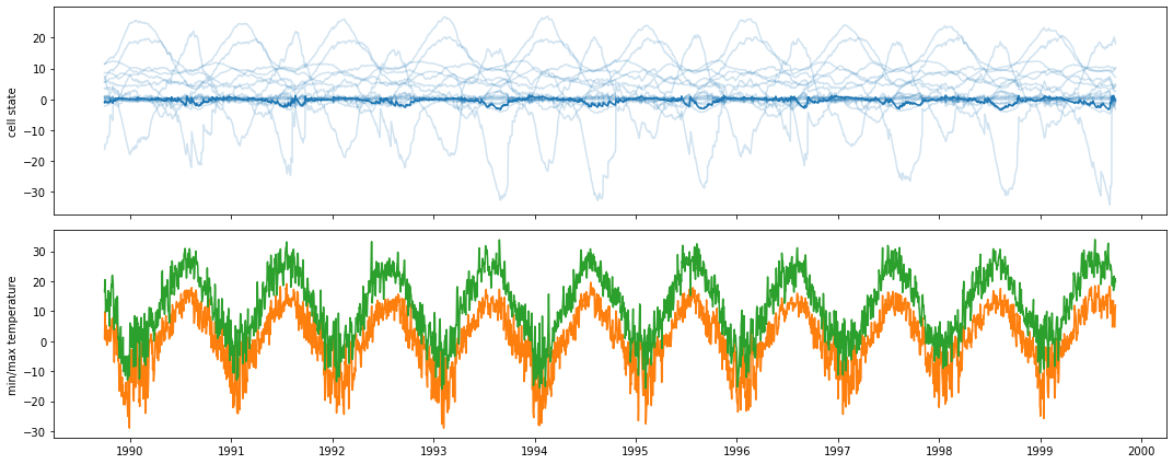
Now, let’s take a closer look at the LSTM states and activations, look at how they evolve over time, and how this evolution correlates with input variables. For instance, cell state 7 quite closely follows the time series of temperature:
[9]:
# Concatenate all batches into one tensor that contains the final time step of each sample.
cell_states = torch.cat([out['c_n'][:, -1, :] for out in customlstm_output], dim=0)

# Load the forcings input for the corresponding date range
date_range = pd.date_range(cudalstm_config.test_start_date, cudalstm_config.test_end_date, freq='1D')
forcings = camelsus.load_camels_us_forcings(cudalstm_config.data_dir, '01022500', 'daymet')[0].loc[date_range]
[10]:
fig, (ax, ax2) = plt.subplots(2, 1, figsize=(15, 6), sharex=True)

ax.plot(date_range, cell_states, c='C0', alpha=.2)
ax.plot(date_range, cell_states[:, 7], c='C0')

ax.set_ylabel('cell state')
ax2.set_ylabel('min/max temperature')

ax2.plot(date_range, forcings['tmin(C)'], c='C1')
ax2.plot(date_range, forcings['tmax(C)'], c='C2')
plt.tight_layout()
Finally, let’s look at how the cell and hidden states and the gate activations develop while the LSTM processes the input sequence of a single sample:
[11]:
f, ax = plt.subplots(4, 2, figsize=(20, 14), sharex=True)
ax[0,0].set_title('Input values')
lines = ax[0,0].plot(dataset[0]['x_d'])  # these are the normalized inputs we fed the LSTM above
ax[0,0].legend(lines, cudalstm_config.dynamic_inputs, frameon=False)

ax[1,0].set_title('Cell state')
ax[1,0].plot(customlstm_output[0]['c_n'][0])

ax[0,1].set_title('Hidden state')
ax[0,1].plot(customlstm_output[0]['h_n'][0])

ax[1,1].set_title('Output gate')
ax[1,1].plot(customlstm_output[0]['o'][0])

ax[2,0].set_title('Forget gate')
ax[2,0].plot(customlstm_output[0]['f'][0])

ax[2,1].set_title('Input gate')
ax[2,1].plot(customlstm_output[0]['i'][0])

ax[3,0].set_title('Cell input activation')
ax[3,0].plot(customlstm_output[0]['g'][0])

f.delaxes(ax[3,1])
plt.tight_layout()
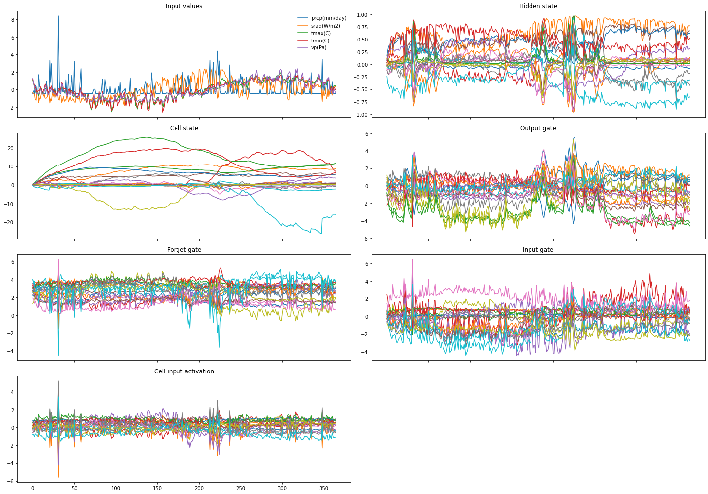
These plots show some interesting characteristics: e.g., the cell states start to behave differently around step 210, and the gates show noticeable activity also around steps 25 and 220 which nicely coincides with high-precipitation events.
That’s it for this tutorial. The verbosity of CustomLSTM’s output gives you lots of options, and we’ll leave it to your imagination as to how you want to analyze the LSTM states and activations. For instance, search for states (or combinations thereof) that correspond to physically meaningful variables, or analyze patterns in the gates’ activations.